
PhD research · Mathematical Programming, 2026
Trust-region methods when curvature estimates blow up
How much work does a trust-region method need when the curvature estimates it relies on are allowed to grow without bound? We give sharp answers, which also address a question raised by Michael Powell in 2010.
Trust-region methods are among the most reliable algorithms for minimizing a function. At each step they replace the function by a simple local model, which they only trust in a small neighborhood. The model needs an estimate of the function's curvature, and in practice this estimate is often computed with quasi-Newton formulas, which are cheap but can grow without limit. Existing guarantees assume that the estimates stay bounded. We show that trust-region methods still work when they do not, and we compute exactly how much the growth costs: the faster the estimates grow, the more work is needed in the worst case, and our bounds cannot be improved.
How a trust-region method works
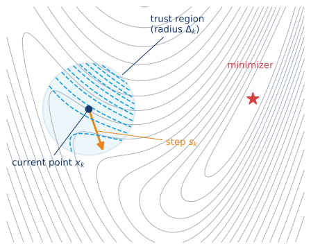
Imagine walking down a mountain in thick fog, trying to reach the lowest point. You can only see the ground around your feet, so you sketch a simple map of the terrain nearby, and you only trust that map up to a certain distance: your trust region. You walk to the lowest point of the map inside that zone. If the real altitude dropped roughly as much as the map predicted, the map was good and you enlarge the zone; if not, you stay put, shrink the zone and try again.
Mathematically, the map is a quadratic model built from the slope (the gradient) and the curvature (the Hessian) of the function at the current point.
Where the difficulty comes from
Computing the exact curvature is often too expensive. Practical implementations approximate it with quasi-Newton updates such as BFGS, SR1 or PSB, which learn the curvature from the steps already taken. They are cheap and work very well in practice, but nothing guarantees that the approximations stay bounded: they may grow as the algorithm proceeds. Almost all worst-case analyses simply assume that they remain bounded.
In 2010, Michael Powell studied trust-region methods whose curvature approximations grow at most linearly with the number of iterations. His convergence proof contained complexity arguments, and he suspected a very pessimistic, double-exponential, worst-case cost.
What we did
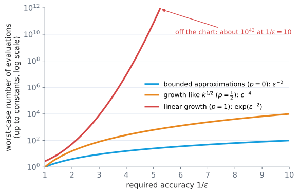
We analyzed a whole family of trust-region methods that contains most known variants, and measured the growth of the curvature approximations with a parameter \(p\):
- \(p = 0\): the approximations stay bounded, the classical situation;
- \(0 < p < 1\): they grow, but more slowly than the number of iterations;
- \(p = 1\): they grow linearly, the case studied by Powell.
For each regime we computed the worst-case number of function evaluations needed to reach a point where the gradient is smaller than a tolerance ε, and built examples showing that these bounds are attained.
- For \(0 \le p < 1\), the cost grows like \(\varepsilon^{-2/(1-p)}\): from the classical \(\varepsilon^{-2}\) when \(p = 0\), to \(\varepsilon^{-4}\) when \(p = 1/2\), and so on.
- For \(p = 1\), the cost grows like \(\exp(c\,\varepsilon^{-2})\): exponential. This is far better than the double exponential Powell suspected, and far worse than other bounds surmised in the literature.
- Similar sharp bounds hold whether growth is measured against the number of accepted steps or against the total number of iterations, and we derive new bounds for convex and strongly convex functions.
Why it matters
Quasi-Newton trust-region methods are used in engineering design, statistics and machine learning. Our results explain why they keep working even when their curvature approximations misbehave, and quantify the price of that misbehavior. They are also the foundation of the analysis of R2N, our method for nonsmooth problems. I presented this work at ICCOPT 2025 in Los Angeles.
For specialists
We consider \(\min_x f(x)\) with \(f \in C^1\), bounded below, with Lipschitz-continuous gradient. At iteration \(k\), the step approximately minimizes \(m_k(s) = f(x_k) + \nabla f(x_k)^T s + \tfrac12 s^T B_k s\) subject to \(\|s\| \le \Delta_k\), with a Cauchy-type decrease condition. Let \(S_{k-1}\) denote the set of successful iterations up to \(k-1\).
- If \(\|B_k\| = O(|S_{k-1}|^p)\) with \(0 \le p < 1\), an ε-stationary point is found after \(O\big([(1-p)\varepsilon^{-2}]^{1/(1-p)}\big)\) evaluations; for \(p = 1\), after \(O(\exp(c_1 \varepsilon^{-2}))\) evaluations. Both bounds are sharp.
- If \(\|B_k\| = O(k^p)\), similar sharp bounds hold for \(0 \le p < 1\). For \(p = 1\) the bound depends on the parameters of the family, and reduces to \(O\big((1 - \log \varepsilon)\exp(c_2 \varepsilon^{-2})\big)\) for the standard trust-region method.