
PhD research · arXiv preprint, 2026
Trust-region methods beyond classical smoothness
Classical guarantees assume that a function's slope never changes faster than a fixed rate. Many functions used in practice, including neural-network losses, break this rule. We analyze trust-region methods under a much weaker assumption.
Almost every convergence guarantee in optimization assumes that the objective is L-smooth: its slope cannot change faster than a fixed rate \(L\), anywhere. Many functions violate this, from simple ones like \(e^x\) or \(x^4\) to the loss functions of neural networks, whose curvature tends to be large exactly where their slope is large. The (L0, L1)-smoothness assumption was introduced to capture this behavior and to explain why tricks such as gradient clipping help train neural networks. In this project we study trust-region methods under a generalized version, (α, L0, L1)-smoothness, and derive worst-case guarantees on the work they need.
When "smooth" is not smooth enough
L-smoothness says that the curvature of the function (its second derivative) is bounded by a constant. That is true for a quadratic, but it already fails for \(f(x) = x^4\) or \(f(x) = e^x\), whose curvature grows without limit. Yet these functions are not wild: their curvature is controlled by their slope. For \(e^x\) the curvature equals the slope; for \(x^4\) it grows like the slope to the power 2/3.
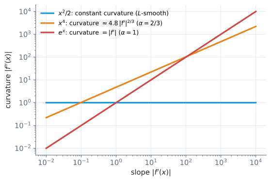
The same phenomenon was observed when training neural networks, for instance language models: in regions where the gradient is large, the curvature is large too. This is the setting in which (L0, L1)-smoothness was proposed.
The assumption
A twice-differentiable function is (α, L0, L1)-smooth when
\[ \|\nabla^2 f(x)\| \;\le\; L_0 + L_1\, \|\nabla f(x)\|^{\alpha} \quad \text{for all } x. \]With \(L_1 = 0\) we recover classical L-smoothness, and α = 1 gives the (L0, L1)-smoothness of Zhang, He, Sra and Jadbabaie (2020). The larger α, the faster curvature is allowed to grow with the slope.
Why trust-region methods are a natural fit
Under this assumption, gradient descent with a fixed step length can overshoot badly where the function is steep. Practitioners therefore clip or normalize the gradient, and in theory the step sizes or clipping thresholds of these methods depend on \(L_0\) and \(L_1\), which are rarely known.
A trust-region method caps the length of every step by the radius of its trust region, and it adjusts that radius automatically by comparing the decrease it predicted with the decrease it obtained. In other words, it has a built-in, adaptive form of step control, and it never needs to know \(L_0\), \(L_1\) or α. (See this project for an illustrated explanation of how trust-region methods work.)
What we study
- Worst-case bounds on the number of iterations and function evaluations that trust-region methods need to reach an approximate stationary point of an (α, L0, L1)-smooth function.
- How these bounds depend on α, \(L_0\) and \(L_1\), and how they compare with the classical L-smooth case.
- How sharp these bounds are, i.e., whether they can be improved.
Why it matters
Deep learning has made (L0, L1)-type assumptions popular, but most analyses concern gradient methods with carefully tuned clipping. Trust-region methods are adaptive by design; understanding their guarantees in this setting helps explain when curvature-aware, self-tuning methods can be used safely on such problems.
For specialists
We consider \(\min_x f(x)\) with \(f\) bounded below and (α, L0, L1)-smooth, and a standard trust-region framework: at iteration \(k\), the step approximately minimizes a quadratic model \(m_k(s) = f(x_k) + \nabla f(x_k)^T s + \tfrac12 s^T B_k s\) subject to \(\|s\| \le \Delta_k\) with a Cauchy decrease condition, the step is accepted according to the ratio of actual to predicted decrease, and \(\Delta_k\) is updated accordingly. None of \(L_0\), \(L_1\), α enters the algorithm. The analysis bounds the number of iterations needed to reach \(\|\nabla f(x_k)\| \le \varepsilon\) in terms of ε, α, \(L_0\) and \(L_1\), and shows that it is tight.